분기한정법(Branch and Bound)은 최적화 문제를 해결하기 위한 효율적인 알고리즘 설계 패러다임이다. 이 방법은 거대한, 때로는 지수적으로 큰 해공간을 체계적으로 탐색하면서 최적해를 찾아내는 강력한 기법이다.
분기한정법은 다양한 최적화 문제를 해결하기 위한 강력하고 유연한 알고리즘 패러다임이다. 이 방법의 핵심은 문제를 체계적으로 나누고, 각 하위 문제의 한계값을 계산하여 유망하지 않은 경로를 가지치기함으로써 탐색 공간을 효과적으로 줄이는 데 있다.
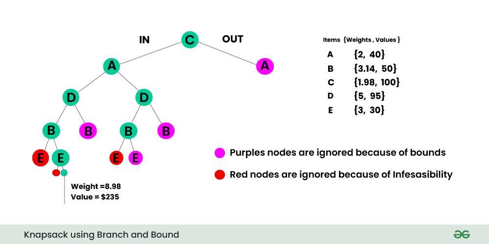
분기한정법은 외판원 문제, 배낭 문제, 작업 할당 문제 등 다양한 NP-hard 최적화 문제에 성공적으로 적용되어 왔다. 물론 최악의 경우에는 여전히 지수 시간이 필요하지만, 효과적인 한계 함수와 가지치기 전략을 통해 실용적인 시간 내에 최적해 또는 근사 최적해를 찾을 수 있다.
현대 컴퓨팅 환경에서는 병렬 처리, 분산 컴퓨팅, 그리고 머신 러닝과 같은 기술의 발전에 힘입어 분기한정법의 활용 범위가 더욱 확장되고 있다. 이러한 발전은 더 큰 규모의 실제 문제를 효율적으로 해결할 수 있는 가능성을 열어주고 있다.
defknapsack_branch_and_bound(weights,values,capacity,index=0,current_weight=0,current_value=0,best_value=0):# 기저 조건: 모든 아이템을 고려했거나 용량을 초과한 경우ifindex==len(weights)orcurrent_weight>capacity:returnbest_value# 현재 아이템을 선택하지 않는 경우best_value=knapsack_branch_and_bound(weights,values,capacity,index+1,current_weight,current_value,best_value)# 현재 아이템을 선택하는 경우ifcurrent_weight+weights[index]<=capacity:new_value=current_value+values[index]ifnew_value>best_value:best_value=new_valuebest_value=knapsack_branch_and_bound(weights,values,capacity,index+1,current_weight+weights[index],new_value,best_value)returnbest_value# 사용 예시weights=[10,20,30]values=[60,100,120]capacity=50result=knapsack_branch_and_bound(weights,values,capacity)print(f"최대 가치: {result}")
importheapqdefknapsack_branch_and_bound_queue(values,weights,capacity):n=len(values)# 가치/무게 비율에 따라 물건 정렬items=[(values[i],weights[i],i)foriinrange(n)]items.sort(key=lambdax:x[0]/x[1],reverse=True)# 최적해를 저장할 변수들best_value=0best_solution=[0]*n# 상한값 계산 함수defbound(k,current_weight,current_value):# (앞의 예제와 동일)ifcurrent_weight>=capacity:return0bound_value=current_valuetotal_weight=current_weightidx=kwhileidx<nandtotal_weight+items[idx][1]<=capacity:bound_value+=items[idx][0]total_weight+=items[idx][1]idx+=1ifidx<n:bound_value+=(capacity-total_weight)*(items[idx][0]/items[idx][1])returnbound_value# 초기 노드 생성# (노드 형식: (-상한값, 물건 인덱스, 현재 무게, 현재 가치, 선택 상태))# 우선순위 큐에서 최대 상한값을 가진 노드를 먼저 처리하기 위해 상한값에 음수 부호를 사용bound_value=bound(0,0,0)priority_queue=[(-bound_value,0,0,0,[0]*n)]heapq.heapify(priority_queue)whilepriority_queue:# 최대 상한값을 가진 노드 추출_,k,current_weight,current_value,solution=heapq.heappop(priority_queue)# 가지치기: 상한값이 현재 최적해보다 작거나 같으면 탐색 중단if-_<=best_value:continue# 모든 물건을 고려했을 때ifk==n:ifcurrent_value>best_value:best_value=current_valuebest_solution=solution[:]continue# 현재 물건 정보item_value,item_weight,original_index=items[k]# 현재 물건을 선택하는 경우 (왼쪽 분기)ifcurrent_weight+item_weight<=capacity:new_solution=solution[:]new_solution[original_index]=1new_value=current_value+item_valuenew_weight=current_weight+item_weightbound_value=bound(k+1,new_weight,new_value)# 가지치기 전에 상한값 확인ifbound_value>best_value:heapq.heappush(priority_queue,(-bound_value,k+1,new_weight,new_value,new_solution))# 현재 물건을 선택하지 않는 경우 (오른쪽 분기)new_solution=solution[:]new_solution[original_index]=0bound_value=bound(k+1,current_weight,current_value)# 가지치기 전에 상한값 확인ifbound_value>best_value:heapq.heappush(priority_queue,(-bound_value,k+1,current_weight,current_value,new_solution))returnbest_value,best_solution
이 구현에서는 우선순위 큐를 사용하여 항상 가장 유망한(상한값이 높은) 노드를 먼저 탐색한다.
defsolve_tsp(distance_matrix):n=len(distance_matrix)classNode:def__init__(self,path,cost,bound):self.path=path# 현재까지의 경로self.cost=cost# 현재까지의 비용self.bound=bound# 하한 값def__lt__(self,other):returnself.bound<other.bounddefcompute_bound(node):# 하한값 계산: 현재 비용 + 각 미방문 도시에서의 최소 비용iflen(node.path)==n:# 모든 도시 방문 완료returnnode.cost+distance_matrix[node.path[-1]][node.path[0]]bound=node.costvisited=set(node.path)current_city=node.path[-1]# 각 미방문 도시에 대해 최소 비용 간선 추가foriinrange(n):ifinotinvisited:min_edge=float('inf')forjinrange(n):ifj!=iandjnotinvisited:min_edge=min(min_edge,distance_matrix[i][j])bound+=min_edgereturnbound# 시작 노드 (0번 도시부터 시작)start_node=Node([0],0,0)start_node.bound=compute_bound(start_node)queue=PriorityQueue()queue.put(start_node)best_tour=Nonebest_cost=float('inf')whilenotqueue.empty():node=queue.get()ifnode.bound>=best_cost:continueiflen(node.path)==n:# 모든 도시 방문# 출발점으로 돌아가는 비용 추가total_cost=node.cost+distance_matrix[node.path[-1]][node.path[0]]iftotal_cost<best_cost:best_cost=total_costbest_tour=node.path+[node.path[0]]else:current_city=node.path[-1]fornext_cityinrange(n):ifnext_citynotinnode.path:new_path=node.path+[next_city]new_cost=node.cost+distance_matrix[current_city][next_city]new_node=Node(new_path,new_cost,0)new_node.bound=compute_bound(new_node)ifnew_node.bound<best_cost:queue.put(new_node)returnbest_tour,best_cost
defsolve_knapsack(values,weights,capacity):n=len(values)classNode:def__init__(self,level,value,weight,bound):self.level=level# 현재 고려 중인 아이템 레벨self.value=value# 현재까지의 가치self.weight=weight# 현재까지의 무게self.bound=bound# 상한 값def__lt__(self,other):returnself.bound>other.bound# 최대화 문제이므로 내림차순defcompute_bound(node):# 이미 무게 제한 초과시 유효하지 않음ifnode.weight>capacity:return0# 현재까지의 가치를 기준값으로 설정bound=node.valuej=node.leveltotal_weight=node.weight# 남은 아이템을 가치/무게 비율이 높은 순서대로 추가whilej<nandtotal_weight+weights[j]<=capacity:bound+=values[j]total_weight+=weights[j]j+=1# 마지막 아이템은 비율에 따라 부분적으로 추가ifj<n:bound+=(capacity-total_weight)*(values[j]/weights[j])returnbound# 가치/무게 비율에 따라 아이템 정렬items=[(values[i],weights[i],i)foriinrange(n)]items.sort(key=lambdax:x[0]/x[1],reverse=True)# 정렬된 순서에 맞게 값 재배치sorted_values=[item[0]foriteminitems]sorted_weights=[item[1]foriteminitems]# 시작 노드start_node=Node(0,0,0,0)start_node.bound=compute_bound(start_node)queue=PriorityQueue()queue.put(start_node)best_value=0best_solution=[]whilenotqueue.empty():node=queue.get()ifnode.bound<=best_value:continue# 모든 아이템 고려 완료ifnode.level==n:ifnode.value>best_value:best_value=node.valuebest_solution=[items[i][2]foriinrange(n)ifnode.included[i]]else:# 현재 아이템을 포함하는 경우include_weight=node.weight+sorted_weights[node.level]ifinclude_weight<=capacity:include_node=Node(node.level+1,node.value+sorted_values[node.level],include_weight,0)include_node.included=node.included+[True]include_node.bound=compute_bound(include_node)ifinclude_node.bound>best_value:queue.put(include_node)# 현재 아이템을 포함하지 않는 경우exclude_node=Node(node.level+1,node.value,node.weight,0)exclude_node.included=node.included+[False]exclude_node.bound=compute_bound(exclude_node)ifexclude_node.bound>best_value:queue.put(exclude_node)returnbest_value,best_solution
defsolve_assignment(cost_matrix):n=len(cost_matrix)classNode:def__init__(self,level,assignments,cost,bound):self.level=level# 현재 할당 중인 작업자self.assignments=assignments# 현재까지의 할당 상태self.cost=cost# 현재까지의 비용self.bound=bound# 하한 값def__lt__(self,other):returnself.bound<other.bounddefcompute_bound(node):# 현재까지의 비용을 기준값으로 설정bound=node.cost# 각 미할당 작업에 대해 최소 비용 추가assigned_tasks=set(node.assignments)foriinrange(node.level,n):min_cost=float('inf')forjinrange(n):ifjnotinassigned_tasks:min_cost=min(min_cost,cost_matrix[i][j])bound+=min_costreturnbound# 시작 노드start_node=Node(0,[],0,0)start_node.bound=compute_bound(start_node)queue=PriorityQueue()queue.put(start_node)best_assignment=Nonebest_cost=float('inf')whilenotqueue.empty():node=queue.get()ifnode.bound>=best_cost:continue# 모든 작업자에게 할당 완료ifnode.level==n:ifnode.cost<best_cost:best_cost=node.costbest_assignment=node.assignments.copy()else:# 현재 작업자에게 각 미할당 작업 할당 시도assigned_tasks=set(node.assignments)fortaskinrange(n):iftasknotinassigned_tasks:new_assignments=node.assignments+[task]new_cost=node.cost+cost_matrix[node.level][task]new_node=Node(node.level+1,new_assignments,new_cost,0)new_node.bound=compute_bound(new_node)ifnew_node.bound<best_cost:queue.put(new_node)returnbest_assignment,best_cost
상태 표현(State Representation) 상태 표현은 문제 해결 과정에서 현재까지의 결정과 남은 선택지를 효과적으로 나타내는 방법이다.
Branch and Bound 알고리즘에서 상태 표현은 다음과 같은 중요한 역할을 한다:
문제 공간 표현: 가능한 모든 해결책(solution space)을 체계적으로 표현한다. 탐색 진행 상황 추적: 알고리즘이 문제 공간을 탐색하는 과정에서 현재 위치를 나타낸다. 한계값(bound) 계산 지원: 각 상태에서 가능한 최적값의 상한 또는 하한을 계산할 수 있게 한다. 가지치기(pruning) 결정 기반: 더 이상 탐색할 가치가 없는 상태를 식별하는 데 사용된다. 상태 표현의 주요 특성 및 고려 사항 상태 표현의 완전성(Completeness)
상태 표현은 문제의 모든 가능한 해결책을 표현할 수 있어야 한다.
불완전한 상태 표현은 최적해를 놓치게 할 수 있다.
...
Branching Strategies
Branching Strategies Branch and Bound(분기한정법)은 조합 최적화 문제를 해결하기 위한 알고리즘 패러다임으로, 가능한 해결책의 공간을 체계적으로 탐색하여 최적의 해를 찾는 방법이다.
이 알고리즘의 핵심 요소 중 하나가 바로 ‘분기 전략(Branching Strategies)‘이다.
분기 전략은 문제 공간을 어떻게 분할하고 탐색할 것인지를 결정하며, 이는 알고리즘의 효율성과 성능에 직접적인 영향을 미친다.
문제 구조를 이해하고 적절한 분기 전략을 선택하는 것은 효율적인 알고리즘 구현을 위해 필수적이다. 변수 기반, 제약 기반, 문제 특화 분기 등 다양한 전략을 이해하고, 문제의 특성에 맞게 적용하거나 조합하는 능력이 중요하다.
...
Branch and Bound vs. Backtracking
Back Tracking vs. Branch and Bound 백트래킹(Backtracking)과 분기한정법(Branch and Bound)은 조합 최적화 문제를 해결하기 위한 두 가지 중요한 알고리즘 설계 패러다임이다.
두 기법 모두 모든 가능한 해결책을 체계적으로 탐색하지만, 그 접근 방식과 최적화 전략에는 중요한 차이가 있다.
백트래킹과 분기한정법은 조합 최적화 문제를 해결하기 위한 강력한 도구이다.
백트래킹은 제약 충족 문제에 더 적합하며, 가능한 모든 해결책이나 첫 번째 유효한 해결책을 찾는 데 중점을 둔다. 반면 분기한정법은 최적화 문제에 더 적합하며, 경계값을 사용하여 최적해를 효율적으로 찾는 데 중점을 둔다.
...
한계 함수(Bounding Functions)
한계 함수(Bounding Functions) Branch and Bound(분기한정법)은 조합 최적화 문제를 해결하기 위한 강력한 알고리즘 패러다임으로, 이 알고리즘의 핵심 요소 중 하나가 바로 ‘한계 함수(Bounding Functions)‘이다.
한계 함수는 분기한정법의 효율성을 결정짓는 중요한 요소로, 불필요한 탐색을 줄이고 최적해를 빠르게 찾는 데 결정적인 역할을 한다.
한계 함수(Bounding Functions)는 Branch and Bound 알고리즘의 핵심 요소로, 불필요한 해공간 탐색을 줄이고 최적해를 효율적으로 찾는 데 중요한 역할을 한다. 효과적인 한계 함수는 정확성, 강도, 계산 효율성, 단조성 등의 특성을 가져야 한다.
...