분기 한정법 (Branch and Bound)

분기한정법(Branch and Bound)은 최적화 문제를 해결하기 위한 효율적인 알고리즘 설계 패러다임이다.
이 방법은 거대한, 때로는 지수적으로 큰 해공간을 체계적으로 탐색하면서 최적해를 찾아내는 강력한 기법이다.

분기한정법은 다양한 최적화 문제를 해결하기 위한 강력하고 유연한 알고리즘 패러다임이다.
이 방법의 핵심은 문제를 체계적으로 나누고, 각 하위 문제의 한계값을 계산하여 유망하지 않은 경로를 가지치기함으로써 탐색 공간을 효과적으로 줄이는 데 있다.

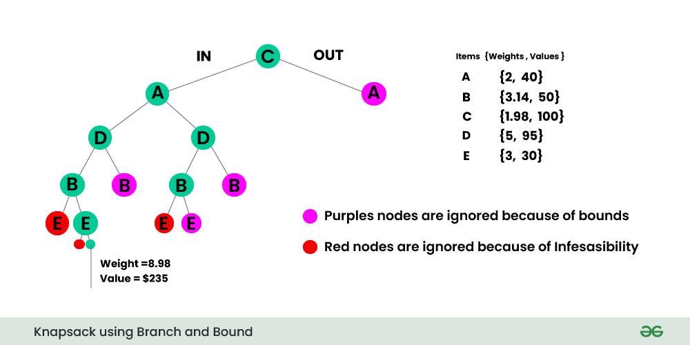
분기한정법은 외판원 문제, 배낭 문제, 작업 할당 문제 등 다양한 NP-hard 최적화 문제에 성공적으로 적용되어 왔다.
물론 최악의 경우에는 여전히 지수 시간이 필요하지만, 효과적인 한계 함수와 가지치기 전략을 통해 실용적인 시간 내에 최적해 또는 근사 최적해를 찾을 수 있다.

현대 컴퓨팅 환경에서는 병렬 처리, 분산 컴퓨팅, 그리고 머신 러닝과 같은 기술의 발전에 힘입어 분기한정법의 활용 범위가 더욱 확장되고 있다. 이러한 발전은 더 큰 규모의 실제 문제를 효율적으로 해결할 수 있는 가능성을 열어주고 있다.

분기 한정법의 기본 개념

분기 한정법은 ‘분기(Branch)‘와 ‘한정(Bound)‘이라는 두 가지 핵심 동작을 결합한 알고리즘이다.

분기(Branch)

분기는 문제를 작은 부분 문제로 나누어 탐색 공간을 확장하는 과정을 의미한다.

한정(Bound)

한정은 각 하위 문제의 해결 가능성을 평가하고 불필요한 탐색을 제거하는 과정이다.

분기와 한정의 상호작용

  1. 분기 과정에서 생성된 각 하위 문제에 대해 한정 과정을 적용한다.
  2. 한정 과정에서 유망하지 않다고 판단된 노드의 하위 트리는 더 이상 탐색하지 않는다.
  3. 가장 유망한 노드를 선택하여 다음 분기를 수행한다.

분기 한정법의 작동 원리

분기 한정법은 다음과 같은 단계로 진행된다:

  1. 초기화: 초기 문제를 설정하고, 최적해의 초기값을 설정한다(최대화 문제의 경우 음의 무한대, 최소화 문제의 경우 양의 무한대).
  2. 분기: 현재 문제를 여러 부분 문제로 나눈다.
  3. 한계값 계산: 각 부분 문제에 대한 한계값을 계산한다.
  4. 가지치기: 한계값이 현재까지의 최적해보다 더 나쁜 부분 문제는 탐색하지 않는다.
  5. 탐색: 가지치기되지 않은 부분 문제들을 특정 순서(일반적으로 최선 우선 탐색)로 계속 탐색한다.
  6. 종료: 모든 부분 문제가 탐색되거나 가지치기될 때까지 반복한다.

분기 한정법의 핵심 구성 요소

분기 한정법을 구현할 때 다음 구성 요소를 고려해야 한다:

상태 표현(State Representation)

문제의 각 상태를 어떻게 표현할지 정의한다.
0-1 배낭 문제에서는 현재 고려 중인 물건의 인덱스, 현재까지 선택한 물건들의 총 무게와 가치, 그리고 선택 상태를 나타내는 배열이 필요하다.

분기 전략(Branching Strategy)

문제를 어떻게 부분 문제로 나눌지 결정한다. 일반적으로 이진 분기(선택함/선택 안함)가 많이 사용되지만, 문제에 따라 다양한 방식이 가능하다.

한계값 함수(Bounding Function)

한계 함수(Bounding Function)는 분기한정법의 효율성을 결정하는 핵심 요소.

좋은 한계 함수는 다음과 같은 특성을 가져야 한다:

  1. 효율성: 빠르게 계산할 수 있어야 한다.
  2. 정확성: 실제 최적값에 가까울수록 더 효과적.
  3. 단조성: 트리를 따라 내려갈수록 더 정확해져야 한다.

한계 함수는 문제의 특성에 따라 다양하게 설계될 수 있으며, 일반적으로 다음과 같은 방법으로 도출된다:

  1. 완화(Relaxation): 문제의 일부 제약 조건을 완화하여 더 쉽게 해결할 수 있는 문제로 변환
  2. 라그랑지안 완화(Lagrangian Relaxation): 제약 조건을 목적 함수에 페널티 항으로 통합
  3. 선형 프로그래밍 완화(Linear Programming Relaxation): 정수 제약을 완화하여 선형 프로그래밍 문제로 해결

탐색 전략(Search Strategy)

분기한정법에서 사용되는 주요 탐색 전략은 다음과 같다:

  1. 최상 우선 탐색(Best-First Search)
    최상 우선 탐색은 하한/상한이 가장 유망한(promising) 노드를 먼저 탐색한다.
    이 방법은 최적해를 더 빨리 찾을 가능성이 높지만, 우선순위 큐를 관리해야 하는 추가 오버헤드가 있다.

  2. 깊이 우선 탐색(Depth-First Search)
    깊이 우선 탐색은 가능한 한 깊이 탐색한 후, 막다른 길에 도달하면 백트래킹한다.
    이 방법은 메모리 효율적이지만, 최적해를 늦게 발견할 수 있다.

  3. 너비 우선 탐색(Breadth-First Search)
    너비 우선 탐색은 레벨별로 모든 노드를 탐색한다. 이 방법은 특정 조건에서 최적해를 보장할 수 있지만, 메모리 요구사항이 매우 높다.

  4. 최소 하한 탐색(Least Lower Bound)
    최소 하한 탐색은 하한이 가장 작은 노드를 먼저 탐색하는 방법이다. 이 방법은 최적해에 빨리 도달할 가능성이 높다.

분기 한정법의 장단점

장점

  1. 최적해 보장: 분기 한정법은 최적해를 보장한다. 가지치기를 통해 일부 경로를 건너뛰지만, 최적해가 포함된 경로는 절대 가지치기되지 않는다.
  2. 효율성: 효과적인 가지치기를 통해 전체 탐색 공간 중 작은 부분만 탐색하므로, 완전 탐색보다 훨씬 효율적이다.
  3. 유연성: 다양한 최적화 문제에 적용할 수 있으며, 문제의 특성에 맞게 한계값 함수와 탐색 전략을 조정할 수 있다.

단점

  1. 최악의 경우 복잡성: 최악의 경우(가지치기가 거의 발생하지 않는 경우), 여전히 모든 가능한 해결책을 탐색해야 할 수 있다.
  2. 한계값 함수의 의존성: 알고리즘의 효율성은 한계값 함수의 정확성과 계산 속도에 크게 의존합니다. 정확하지만 계산이 복잡한 한계값 함수는 오히려 전체 성능을 저하시킬 수 있다.
  3. 메모리 요구사항: 특히 큐 기반 구현에서는 많은 노드를 메모리에 저장해야 할 수 있어 큰 문제에서는 메모리 부족 문제가 발생할 수 있다.

분기한정법의 시간 및 공간 복잡도

분기한정법의 효율성은 문제의 특성, 한계 함수의 품질, 그리고 가지치기의 효과에 크게 의존한다.

분기한정법의 향상 기법

분기한정법의 성능을 더욱 향상시키기 위한 여러 기법들이 연구되어 왔다:

  1. 지배 관계(Dominance Relations)
    어떤 노드가 다른 노드를 지배한다면(항상 더 나은 해결책을 제공), 열등한 노드는 탐색에서 제외할 수 있다.

  2. 휴리스틱 함수(Heuristic Functions)
    초기 해결책을 빠르게 찾거나, 탐색 순서를 개선하기 위해 휴리스틱 함수를 사용할 수 있다.

  3. 병렬 처리(Parallelization)
    독립적인 하위 문제들을 여러 프로세서에서 병렬로 처리하여 성능을 향상시킬 수 있다.

  4. 메모이제이션(Memoization)
    이미 탐색한 상태를 저장하여 중복 계산을 피할 수 있다.

  5. 구조적 특성 활용(Exploiting Problem Structure)
    문제의 특수한 구조적 특성을 활용하여 더 효과적인 한계 함수를 설계할 수 있다.

분기 한정법 구현 시 주의사항

분기 한정법을 효과적으로 구현하기 위한 몇 가지 주의사항:

  1. 한계값 함수의 균형: 계산이 간단하면서도 정확한 한계값 함수를 설계해야 한다. 너무 느슨한 한계값은 가지치기 효과가 적고, 너무 복잡한 계산은 오버헤드가 크다.
  2. 메모리 관리: 특히 큐 기반 구현에서는 메모리 사용량에 주의해야 한다. 노드 생성과 저장을 최적화하는 전략이 필요할 수 있다.
  3. 초기 해결책: 가능하면 탐색 시작 전에 좋은 초기 해결책을 구하여 가지치기 효과를 극대화한다.
  4. 문제 특성 활용: 문제의 구조와 특성을 분석하여 더 효과적인 분기 전략과 한계값 함수를 설계한다.

분기한정법의 구현

기본 방식

 1
 2
 3
 4
 5
 6
 7
 8
 9
10
11
12
def branch_and_bound(현재_상태):
    if 목표_달성(현재_상태):
        결과_저장(현재_상태)
        return
    
    if not 유망성_검사(현재_상태):
        return  # 가지치기
    
    for 다음_선택 in 가능한_선택들:
        상태_변경(현재_상태, 다음_선택)
        branch_and_bound(현재_상태)
        상태_복구(현재_상태)

분기 한정법은 크게 두 가지 방식으로 구현된다:

재귀적 구현(Recursive Implementation)

재귀 함수를 사용하여 구현한다. 이 방식은 깊이 우선 탐색을 기반으로 하며, 구현이 직관적이고 간단하다.

 1
 2
 3
 4
 5
 6
 7
 8
 9
10
11
12
13
14
15
16
17
18
19
20
21
22
23
24
def knapsack_branch_and_bound(weights, values, capacity, index=0, current_weight=0, current_value=0, best_value=0):
    # 기저 조건: 모든 아이템을 고려했거나 용량을 초과한 경우
    if index == len(weights) or current_weight > capacity:
        return best_value

    # 현재 아이템을 선택하지 않는 경우
    best_value = knapsack_branch_and_bound(weights, values, capacity, index + 1, current_weight, current_value, best_value)

    # 현재 아이템을 선택하는 경우
    if current_weight + weights[index] <= capacity:
        new_value = current_value + values[index]
        if new_value > best_value:
            best_value = new_value
        best_value = knapsack_branch_and_bound(weights, values, capacity, index + 1, current_weight + weights[index], new_value, best_value)

    return best_value

# 사용 예시
weights = [10, 20, 30]
values = [60, 100, 120]
capacity = 50

result = knapsack_branch_and_bound(weights, values, capacity)
print(f"최대 가치: {result}")

큐 기반 구현(Queue-based Implementation)

우선순위 큐를 사용하여 구현하는 방식으로, 최선 우선 탐색을 기반으로 한다. 한계값이 가장 유망한 노드를 먼저 탐색하므로 효율성이 높다.

 1
 2
 3
 4
 5
 6
 7
 8
 9
10
11
12
13
14
15
16
17
18
19
20
21
22
23
24
25
26
27
28
29
30
31
32
33
34
35
36
37
38
39
40
41
42
43
44
45
46
47
48
49
50
51
52
53
54
55
56
57
58
59
60
61
62
63
64
65
66
67
68
69
70
71
72
73
74
75
76
77
78
79
import heapq

def knapsack_branch_and_bound_queue(values, weights, capacity):
    n = len(values)
    # 가치/무게 비율에 따라 물건 정렬
    items = [(values[i], weights[i], i) for i in range(n)]
    items.sort(key=lambda x: x[0]/x[1], reverse=True)
    
    # 최적해를 저장할 변수들
    best_value = 0
    best_solution = [0] * n
    
    # 상한값 계산 함수
    def bound(k, current_weight, current_value):
        # (앞의 예제와 동일)
        if current_weight >= capacity:
            return 0
        
        bound_value = current_value
        total_weight = current_weight
        idx = k
        
        while idx < n and total_weight + items[idx][1] <= capacity:
            bound_value += items[idx][0]
            total_weight += items[idx][1]
            idx += 1
        
        if idx < n:
            bound_value += (capacity - total_weight) * (items[idx][0] / items[idx][1])
        
        return bound_value
    
    # 초기 노드 생성
    # (노드 형식: (-상한값, 물건 인덱스, 현재 무게, 현재 가치, 선택 상태))
    # 우선순위 큐에서 최대 상한값을 가진 노드를 먼저 처리하기 위해 상한값에 음수 부호를 사용
    bound_value = bound(0, 0, 0)
    priority_queue = [(-bound_value, 0, 0, 0, [0] * n)]
    heapq.heapify(priority_queue)
    
    while priority_queue:
        # 최대 상한값을 가진 노드 추출
        _, k, current_weight, current_value, solution = heapq.heappop(priority_queue)
        
        # 가지치기: 상한값이 현재 최적해보다 작거나 같으면 탐색 중단
        if -_ <= best_value:
            continue
        
        # 모든 물건을 고려했을 때
        if k == n:
            if current_value > best_value:
                best_value = current_value
                best_solution = solution[:]
            continue
        
        # 현재 물건 정보
        item_value, item_weight, original_index = items[k]
        
        # 현재 물건을 선택하는 경우 (왼쪽 분기)
        if current_weight + item_weight <= capacity:
            new_solution = solution[:]
            new_solution[original_index] = 1
            new_value = current_value + item_value
            new_weight = current_weight + item_weight
            bound_value = bound(k + 1, new_weight, new_value)
            
            # 가지치기 전에 상한값 확인
            if bound_value > best_value:
                heapq.heappush(priority_queue, (-bound_value, k + 1, new_weight, new_value, new_solution))
        
        # 현재 물건을 선택하지 않는 경우 (오른쪽 분기)
        new_solution = solution[:]
        new_solution[original_index] = 0
        bound_value = bound(k + 1, current_weight, current_value)
        
        # 가지치기 전에 상한값 확인
        if bound_value > best_value:
            heapq.heappush(priority_queue, (-bound_value, k + 1, current_weight, current_value, new_solution))
    
    return best_value, best_solution

이 구현에서는 우선순위 큐를 사용하여 항상 가장 유망한(상한값이 높은) 노드를 먼저 탐색한다.

분기한정법의 대표적인 적용 사례

분기한정법은 다양한 최적화 문제에 성공적으로 적용되어 왔다.

다음은 가장 잘 알려진 적용 사례들:

외판원 문제(Traveling Salesman Problem, TSP)

외판원 문제는 모든 도시를 한 번씩 방문하고 출발 도시로 돌아오는 최단 경로를 찾는 문제.

 1
 2
 3
 4
 5
 6
 7
 8
 9
10
11
12
13
14
15
16
17
18
19
20
21
22
23
24
25
26
27
28
29
30
31
32
33
34
35
36
37
38
39
40
41
42
43
44
45
46
47
48
49
50
51
52
53
54
55
56
57
58
59
60
61
62
63
64
65
66
67
68
def solve_tsp(distance_matrix):
    n = len(distance_matrix)
    
    class Node:
        def __init__(self, path, cost, bound):
            self.path = path  # 현재까지의 경로
            self.cost = cost  # 현재까지의 비용
            self.bound = bound  # 하한 값
        
        def __lt__(self, other):
            return self.bound < other.bound
    
    def compute_bound(node):
        # 하한값 계산: 현재 비용 + 각 미방문 도시에서의 최소 비용
        if len(node.path) == n:  # 모든 도시 방문 완료
            return node.cost + distance_matrix[node.path[-1]][node.path[0]]
        
        bound = node.cost
        visited = set(node.path)
        current_city = node.path[-1]
        
        # 각 미방문 도시에 대해 최소 비용 간선 추가
        for i in range(n):
            if i not in visited:
                min_edge = float('inf')
                for j in range(n):
                    if j != i and j not in visited:
                        min_edge = min(min_edge, distance_matrix[i][j])
                bound += min_edge
        
        return bound
    
    # 시작 노드 (0번 도시부터 시작)
    start_node = Node([0], 0, 0)
    start_node.bound = compute_bound(start_node)
    
    queue = PriorityQueue()
    queue.put(start_node)
    
    best_tour = None
    best_cost = float('inf')
    
    while not queue.empty():
        node = queue.get()
        
        if node.bound >= best_cost:
            continue
        
        if len(node.path) == n:  # 모든 도시 방문
            # 출발점으로 돌아가는 비용 추가
            total_cost = node.cost + distance_matrix[node.path[-1]][node.path[0]]
            if total_cost < best_cost:
                best_cost = total_cost
                best_tour = node.path + [node.path[0]]
        else:
            current_city = node.path[-1]
            for next_city in range(n):
                if next_city not in node.path:
                    new_path = node.path + [next_city]
                    new_cost = node.cost + distance_matrix[current_city][next_city]
                    
                    new_node = Node(new_path, new_cost, 0)
                    new_node.bound = compute_bound(new_node)
                    
                    if new_node.bound < best_cost:
                        queue.put(new_node)
    
    return best_tour, best_cost

0-1 배낭 문제(Knapsack Problem)

배낭 문제는 주어진 무게 제한 내에서 최대 가치를 갖는 아이템 조합을 선택하는 문제.

주어진 조건:

목표:

수학적 표현:

1
2
3
최대화: `Σ(v[i] * x[i])  (i = 1 to n)`
제약 조건: `Σ(w[i] * x[i]) ≤ W`
여기서` x[i]는 0 또는 1 (물건을 선택하거나 선택하지 않음)`

0/1 Knapsack using Branch and Bound
Source: https://www.geeksforgeeks.org/0-1-knapsack-using-branch-and-bound/

 1
 2
 3
 4
 5
 6
 7
 8
 9
10
11
12
13
14
15
16
17
18
19
20
21
22
23
24
25
26
27
28
29
30
31
32
33
34
35
36
37
38
39
40
41
42
43
44
45
46
47
48
49
50
51
52
53
54
55
56
57
58
59
60
61
62
63
64
65
66
67
68
69
70
71
72
73
74
75
76
77
78
79
80
81
82
83
84
85
86
def solve_knapsack(values, weights, capacity):
    n = len(values)
    
    class Node:
        def __init__(self, level, value, weight, bound):
            self.level = level  # 현재 고려 중인 아이템 레벨
            self.value = value  # 현재까지의 가치
            self.weight = weight  # 현재까지의 무게
            self.bound = bound  # 상한 값
        
        def __lt__(self, other):
            return self.bound > other.bound  # 최대화 문제이므로 내림차순
    
    def compute_bound(node):
        # 이미 무게 제한 초과시 유효하지 않음
        if node.weight > capacity:
            return 0
        
        # 현재까지의 가치를 기준값으로 설정
        bound = node.value
        j = node.level
        total_weight = node.weight
        
        # 남은 아이템을 가치/무게 비율이 높은 순서대로 추가
        while j < n and total_weight + weights[j] <= capacity:
            bound += values[j]
            total_weight += weights[j]
            j += 1
        
        # 마지막 아이템은 비율에 따라 부분적으로 추가
        if j < n:
            bound += (capacity - total_weight) * (values[j] / weights[j])
        
        return bound
    
    # 가치/무게 비율에 따라 아이템 정렬
    items = [(values[i], weights[i], i) for i in range(n)]
    items.sort(key=lambda x: x[0]/x[1], reverse=True)
    
    # 정렬된 순서에 맞게 값 재배치
    sorted_values = [item[0] for item in items]
    sorted_weights = [item[1] for item in items]
    
    # 시작 노드
    start_node = Node(0, 0, 0, 0)
    start_node.bound = compute_bound(start_node)
    
    queue = PriorityQueue()
    queue.put(start_node)
    
    best_value = 0
    best_solution = []
    
    while not queue.empty():
        node = queue.get()
        
        if node.bound <= best_value:
            continue
        
        # 모든 아이템 고려 완료
        if node.level == n:
            if node.value > best_value:
                best_value = node.value
                best_solution = [items[i][2] for i in range(n) if node.included[i]]
        else:
            # 현재 아이템을 포함하는 경우
            include_weight = node.weight + sorted_weights[node.level]
            if include_weight <= capacity:
                include_node = Node(node.level + 1, 
                                    node.value + sorted_values[node.level], 
                                    include_weight, 0)
                include_node.included = node.included + [True]
                include_node.bound = compute_bound(include_node)
                
                if include_node.bound > best_value:
                    queue.put(include_node)
            
            # 현재 아이템을 포함하지 않는 경우
            exclude_node = Node(node.level + 1, node.value, node.weight, 0)
            exclude_node.included = node.included + [False]
            exclude_node.bound = compute_bound(exclude_node)
            
            if exclude_node.bound > best_value:
                queue.put(exclude_node)
    
    return best_value, best_solution

작업 할당 문제(Assignment Problem)

작업 할당 문제는 n개의 작업을 n명의 작업자에게 최소 비용으로 할당하는 문제.

 1
 2
 3
 4
 5
 6
 7
 8
 9
10
11
12
13
14
15
16
17
18
19
20
21
22
23
24
25
26
27
28
29
30
31
32
33
34
35
36
37
38
39
40
41
42
43
44
45
46
47
48
49
50
51
52
53
54
55
56
57
58
59
60
61
62
63
64
def solve_assignment(cost_matrix):
    n = len(cost_matrix)
    
    class Node:
        def __init__(self, level, assignments, cost, bound):
            self.level = level  # 현재 할당 중인 작업자
            self.assignments = assignments  # 현재까지의 할당 상태
            self.cost = cost  # 현재까지의 비용
            self.bound = bound  # 하한 값
        
        def __lt__(self, other):
            return self.bound < other.bound
    
    def compute_bound(node):
        # 현재까지의 비용을 기준값으로 설정
        bound = node.cost
        
        # 각 미할당 작업에 대해 최소 비용 추가
        assigned_tasks = set(node.assignments)
        for i in range(node.level, n):
            min_cost = float('inf')
            for j in range(n):
                if j not in assigned_tasks:
                    min_cost = min(min_cost, cost_matrix[i][j])
            bound += min_cost
        
        return bound
    
    # 시작 노드
    start_node = Node(0, [], 0, 0)
    start_node.bound = compute_bound(start_node)
    
    queue = PriorityQueue()
    queue.put(start_node)
    
    best_assignment = None
    best_cost = float('inf')
    
    while not queue.empty():
        node = queue.get()
        
        if node.bound >= best_cost:
            continue
        
        # 모든 작업자에게 할당 완료
        if node.level == n:
            if node.cost < best_cost:
                best_cost = node.cost
                best_assignment = node.assignments.copy()
        else:
            # 현재 작업자에게 각 미할당 작업 할당 시도
            assigned_tasks = set(node.assignments)
            for task in range(n):
                if task not in assigned_tasks:
                    new_assignments = node.assignments + [task]
                    new_cost = node.cost + cost_matrix[node.level][task]
                    
                    new_node = Node(node.level + 1, new_assignments, new_cost, 0)
                    new_node.bound = compute_bound(new_node)
                    
                    if new_node.bound < best_cost:
                        queue.put(new_node)
    
    return best_assignment, best_cost

실제 응용 사례

분기한정법은 다양한 실제 문제에 응용되고 있다:

  1. 물류 및 운송 최적화
    • 차량 경로 문제(Vehicle Routing Problem)
    • 작업 스케줄링(Job Scheduling)
  2. 네트워크 설계
    • 네트워크 흐름 최적화
    • 통신 네트워크 설계
  3. 자원 할당
    • 프로젝트 스케줄링
    • 인력 배치 최적화
  4. 생산 계획
    • 공정 최적화
    • 재고 관리
  5. 금융 분야
    • 포트폴리오 최적화
    • 위험 최소화 전략

분기한정법의 미래 발전 방향

분기한정법은 계속해서 발전하고 있으며, 다음과 같은 방향으로 연구가 진행되고 있다:

  1. 머신 러닝 통합: 노드 선택 및 분기 전략을 개선하기 위한 머신 러닝 기법 활용
  2. 고급 한계 함수: 더 정확하고 계산 효율적인 한계 함수 개발
  3. 분산 및 병렬 알고리즘: 대규모 문제를 위한 분산 컴퓨팅 방법론
  4. 하이브리드 접근법: 메타휴리스틱, 동적 계획법 등 다른 기법과의 통합

참고 및 출처